Tutorial: Redshift Estimation of High-z Galaxies
Table of Contents
- 1. Redshift
- 2. Photometric Redshift Estimation - Primer
- 3. Spectroscopic Redshifts - Primer
- 3.1. Astrophysical Emission Lines
- 3.2. Emission Lines from galaxies.
- 3.3. Obtaining Redshifts from Emission Lines
- 3.3.1. Spectroscopy
- 3.3.2. 1D Spectrum = Input for Redshift Determination
- 3.3.3. Example / Exercise: Extreme Emission Line Galaxies
- 3.3.4. Example: Stack of VUDS 1D spectra sorted by redshift
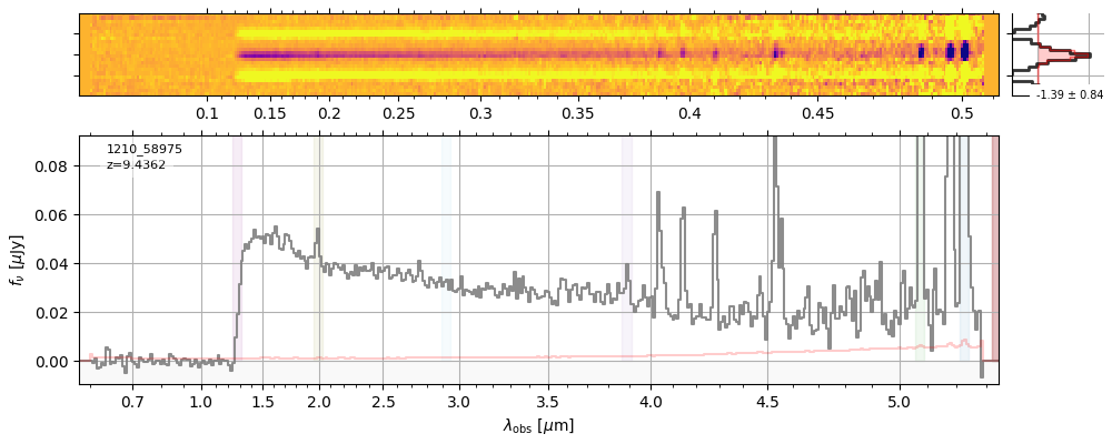
- 3.3.5. Example: Public Archive of JWST Spectra (DJA)
- 3.3.6. Readymade solutions
- 3.3.7. Underlying principle: Minimization
1. Redshift
\[ z_\mathrm{obs} = \frac{\nu_0}{\nu_\mathrm{obs}} - 1 = \frac{\lambda_\mathrm{obs}}{\lambda_0} - 1 \]
Note: \(z_\mathrm{obs}\) is not exactly cosmological redshift \(z_\mathrm{cos}\). In general \(1 + z_\mathrm{obs} = (1 + z_\mathrm{cos}) \cdot (1 + z_\mathrm{perc})\) if local standard at rest is fixed against cosmic microwave background (Davis & Scrimgeour 2014).
See David W. Hogg: "Distance Measures in Cosmology".
Uninitated show "confusion" due to "velocity" in Hubble's Law: \(v = H_0 \cdot d\) (Hubble constant): \(c \cdot z = H_0 \cdot d\) is only valid when \(v/c << 1\). Redshift only appears as recessional velocity, but nothing is really moving away from us (only the scale factor changed while the light was travelling).
2. Photometric Redshift Estimation - Primer
2.1. Imaging Data
All astrophysics begins with imaging.
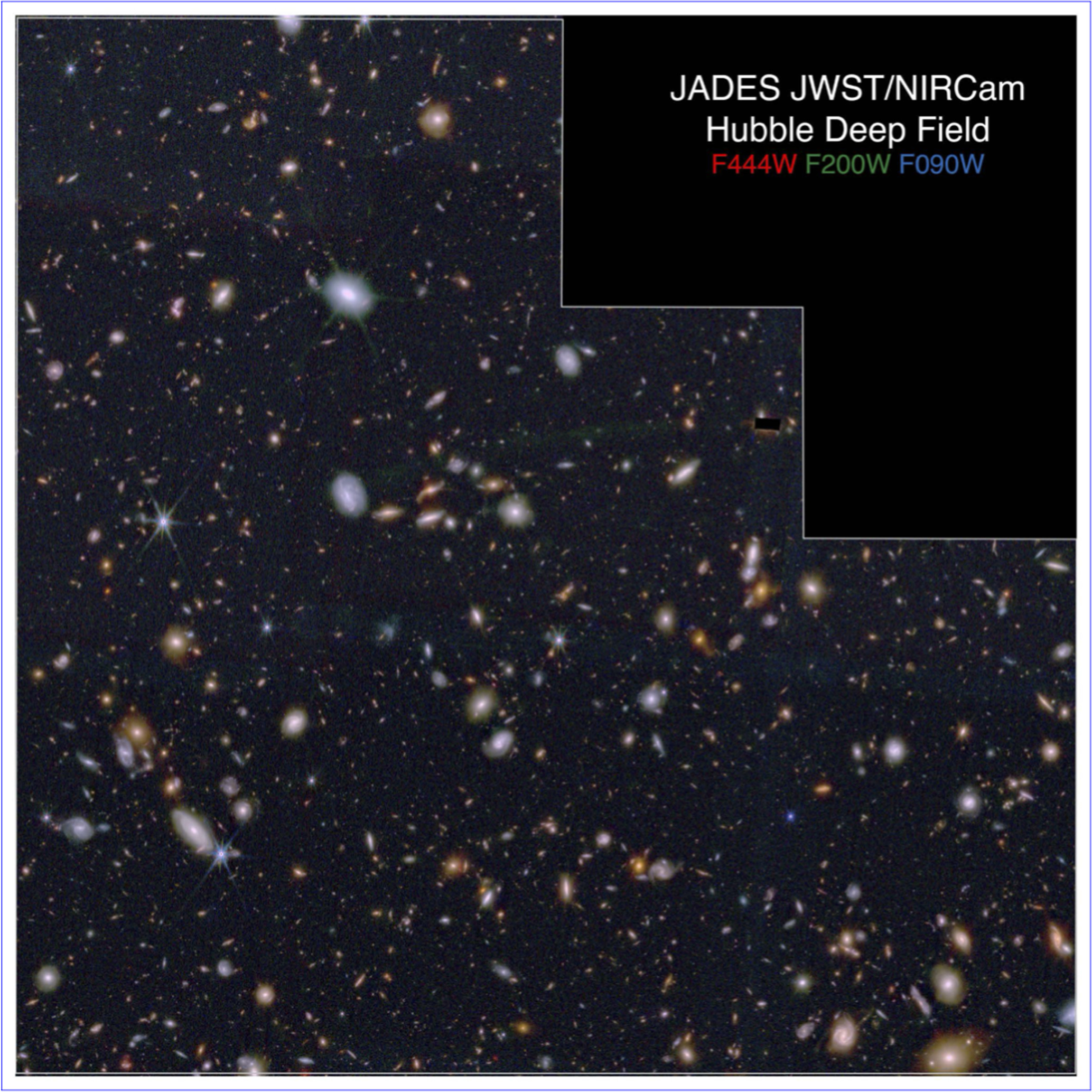 (From D’Eugenio et al 2025 ApJS 277 4.)
- Multiple photometric bands.
- HST: ACS / WFC3.
- JWST: NIRCAM.
- for filter curves, see, e.g., the Asiago Database on Photometric Systems.
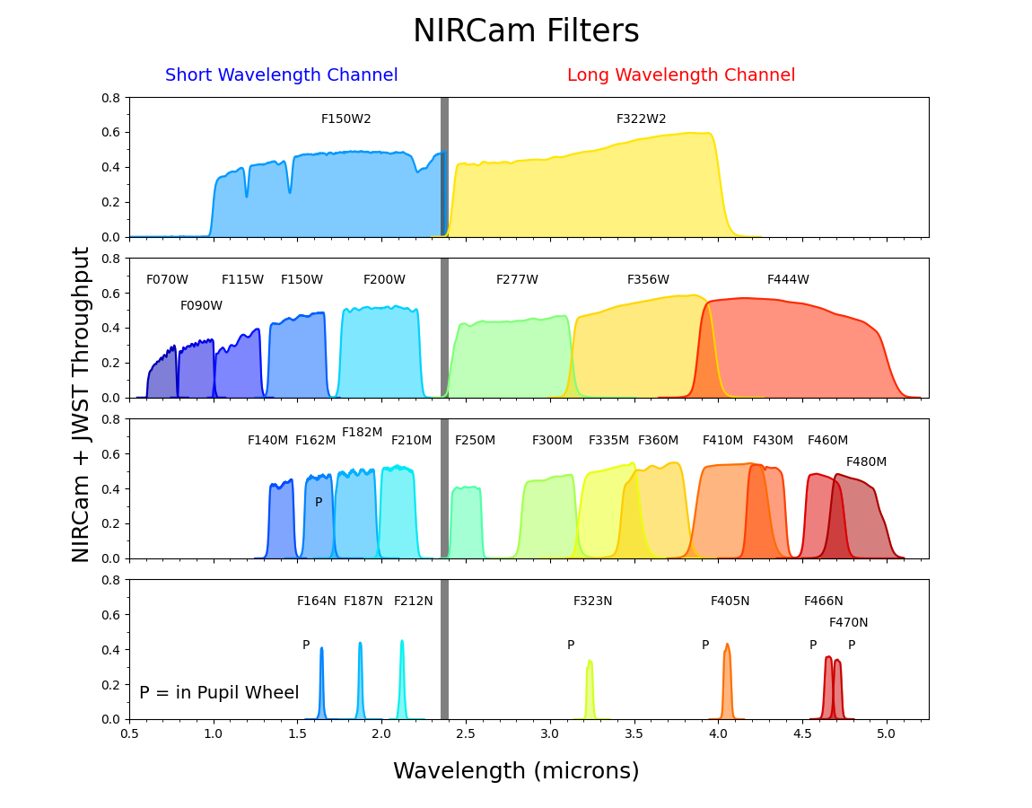
Figure 1: JWST/NIRCam Throughput Curves
- Imaging Sky Surveys - Wedding Cake Strategy
- Wide-Field (≳π sr): LSST, Euclid (Wide), DESI Legacy Survey, SDSS, Pan-STARRS
- Meedium-Deep (~ few to tens sq. deg): Subaru HSSP, CFHT Legacy Survey.
- Deep (Space, HST, now JWST, ∼ 100 arcmin²): GOODS → CANDELS, JWST/CEERS, ASTRODEEP-JWST.
- Ultra-Deep (∼ few arcmin²): Hubble eXtreme Deep Field, JWST/JADES.
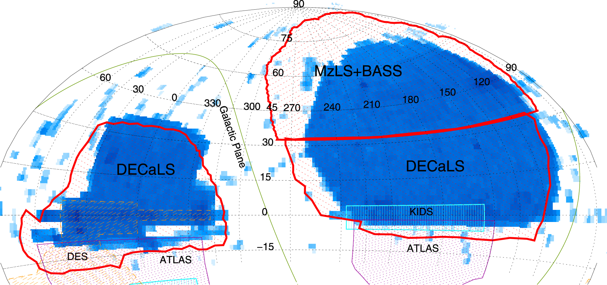 (From Dey et al 2019 AJ 157 168.)
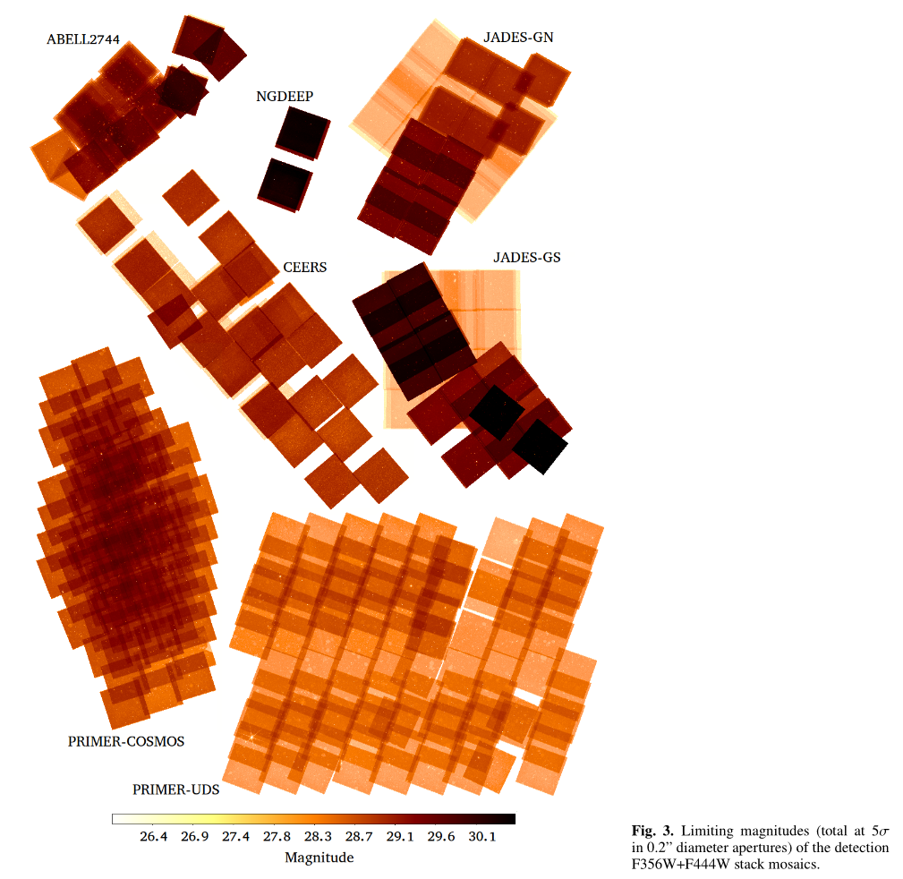 (From
(From 2.2. Source Detection & Measurements (magnitudes)
- Classical — filtering, thresholding, labelling, and flux measurement in
calculated apertures:
- SExtractor (Bertin & Arnouts 1996).
- sep - python implementation of SExtractor algorithms (Barbary 2016).
- photutils (astropy coordinated package) — https://photutils.readthedocs.io
- Modern Approaches — forward modelling images (after detection)
- SᴏᴜʀᴄᴇXᴛʀᴀᴄᴛᴏʀ++ — modern version of SExtractor in C++ incl. model fitting (Bertin et al. 2020).
- The Tractor — https://thetractor.org/
- used in legacysurvey.org
- see .
- ForcePho — https://forcepho.readthedocs.io/ (Johnson et al in prep. since ages) — "weapon of choice for JWST high-z galaxy investigators".
2.2.1. Result: Photometric Catalogue
- source positions (mom1).
- structural paramters (mom2, e.g., major-, and minor-axis ).
- flux densities (total source) in the different bands (classical: in different
apertures). Typical units.
- magnitudes (AB magnitudes).
- flux density (~erg/s/cm²/Ångstrom, or Jy, or W/m²/Hz).
2.2.2. Example: 👁️ Photometric Redshift by Eye 👁️
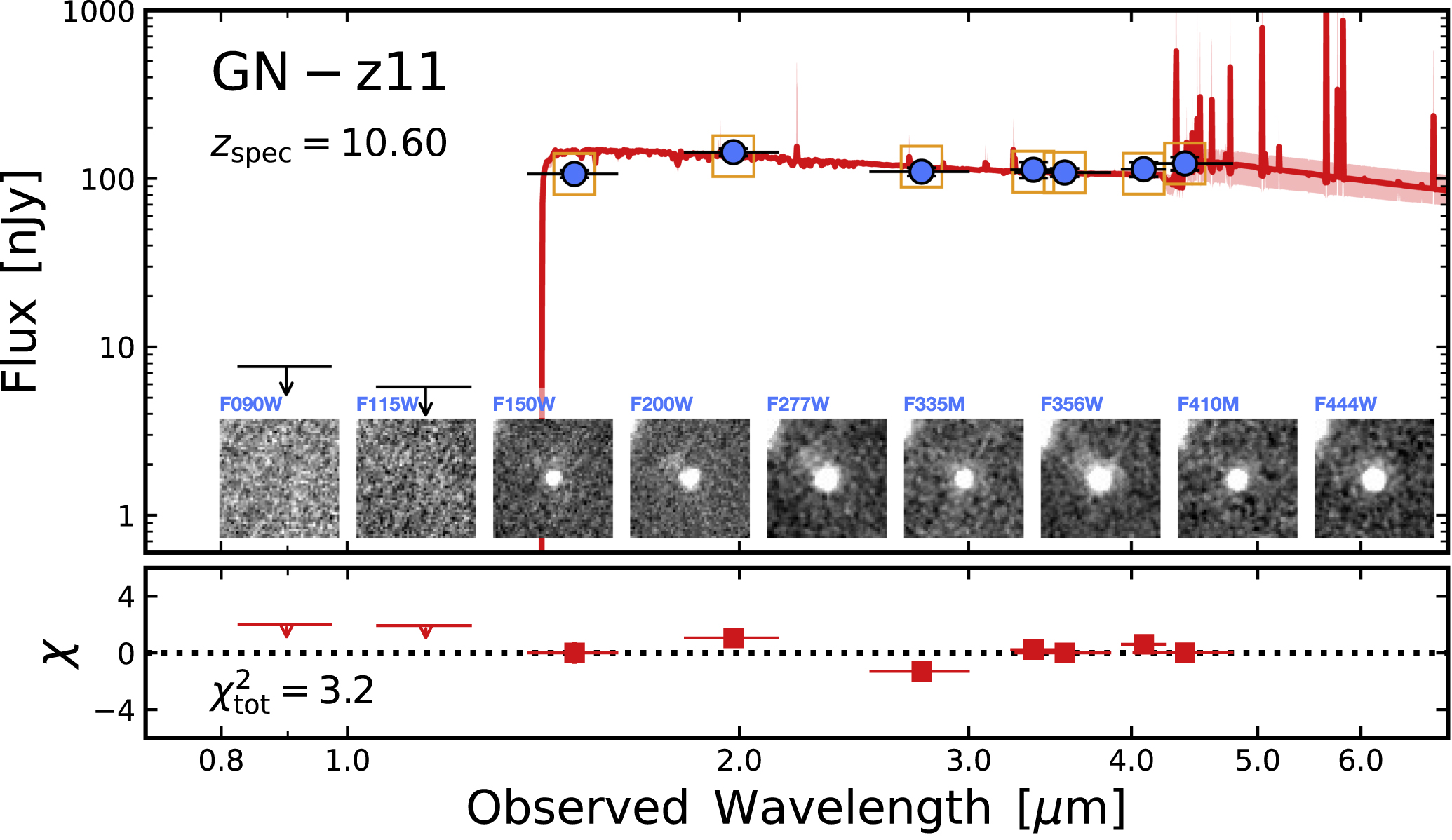 From Tacchella et al. (2023). This galaxy is observed 430 Myr after the Big Bang!
The Lyα break at 1216Å caused by intergalactic medium absorption (Gunn-Peterson trough) must be redward of F115W filter (effective wavelength 1.15μm). The lower limit for the redshift is thus 10.45.
2.2.2.1. Exercises
- Units in the Photometric Catalogue
Curti et al. (2025) present the following photometry for JADES-GS-z9, a z∼9 galaxy: F_ν(F150W) = 49.99 ± 0.34 nJy (their Table 7).
- Calculate F_λ in erg/s/cm²/Angstrom (assume effective wavelength of filter is 1.5μm).
- Calculate m_AB (magnitude in AB system).
- Calculate absolute magnitude M_UV assuming z∼9 and cosmology (ΩΛ=0.7, H0=70km/s/Mpc).
- 👁️ Photometric Redshift by Eye 👁️
Witstok et al. (2025) show the following photometric JWST/NIRCam data (and model, as well as model-residual) for their discovered galaxy.
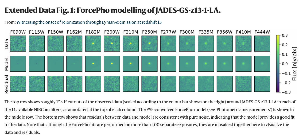
Figure 2: Observational imaging data and flux measurement procedure for early universe galaxy discovered by Witstok et al. (2025).
- Describe the percieved spectral energy distribution from the central source in those images.
- Assume there is a spectral discontinuity in the intrinsic SED at 1216 Å (Lyman-α break), with S(λ<1216Å)=0. What is the redshift of the source? (Hint: Filter names encode the effective wavlength in μm.)
- (Try to understand the astrophysical reason for justifying this assumption of such a spectral "break" at 1216Å.)
- (Photospheric absorption predicts a break at 912Å in spectral energy distributions of stellar atmospheres (Lyman break). Why is this spectral break not relevant here, and how is it related to Lymena break galaxies?)
- Explore the JADES Survey imaging data by eye — https://jades-survey.github.io/viewer/ — and find a possible high-redshift candidate. Check your candidate using the overlay tools on the top right corner.
2.3. From Magnitudes in Bands to Redshifts
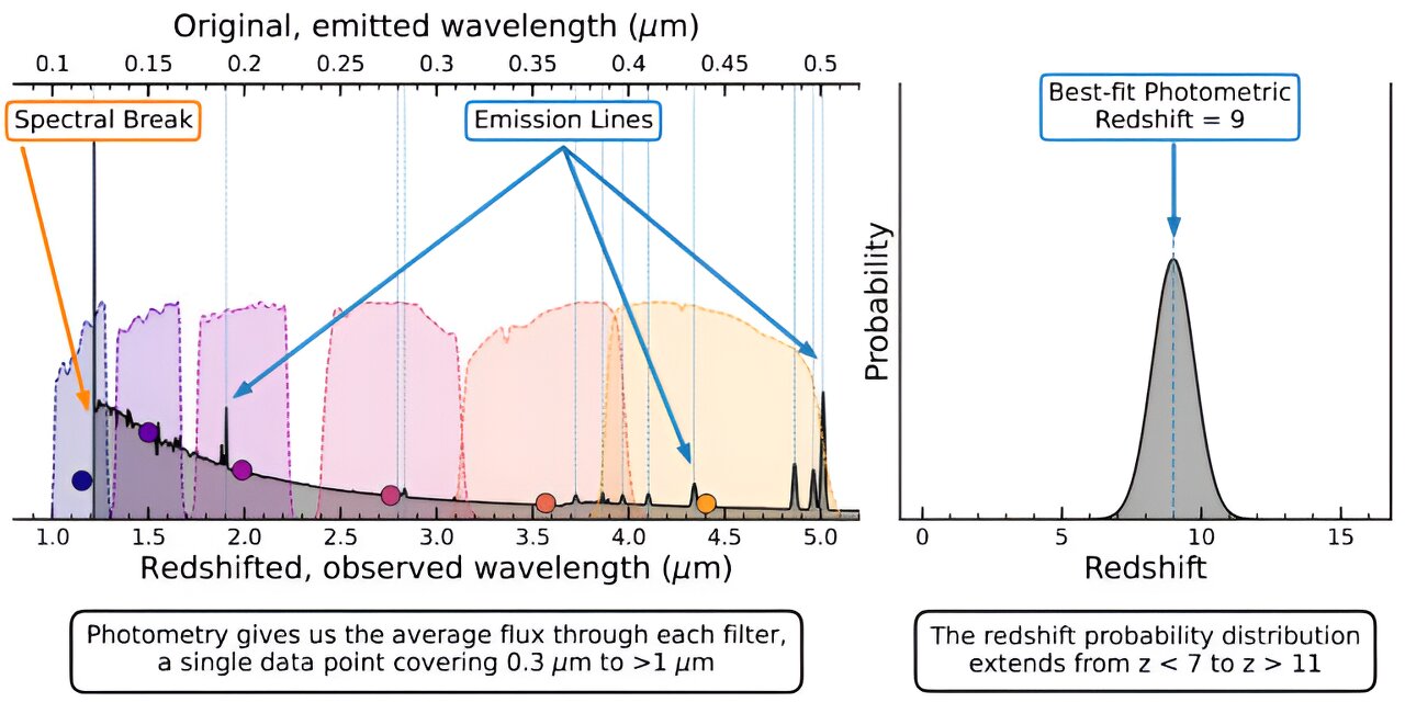
Photometric redshift estimation techniques.
Result: Probability distribution for the redshift of the source.
- Template-based + minimization: e.g., EAZY (Brammer et al. 2008), popular code - used, e.g., in JADES & ASTRODEEP — new python version in the works — https://eazy-py.readthedocs.io/en/latest/
- LePHARE – Templates + Calibrated against spectroscopic redshifts - Baysian methodology (Ilbert et al. 2006). Get from pypi: https://pypi.org/project/lephare/
- Machine-learning based approaches …
- …
(Topic of active research.)
 From phys.org
2.3.1. High-z galaxy example: "Maisie's Galaxy"
- Initial discovery based only on photometric redshift: \(z_\mathrm{phot} = 11.8^{+0.3}_{-0.2}\) (Finkelstein et al 2022 ApJL 940 L55).
Present redshift p(z) distributions from five(!) different codes.
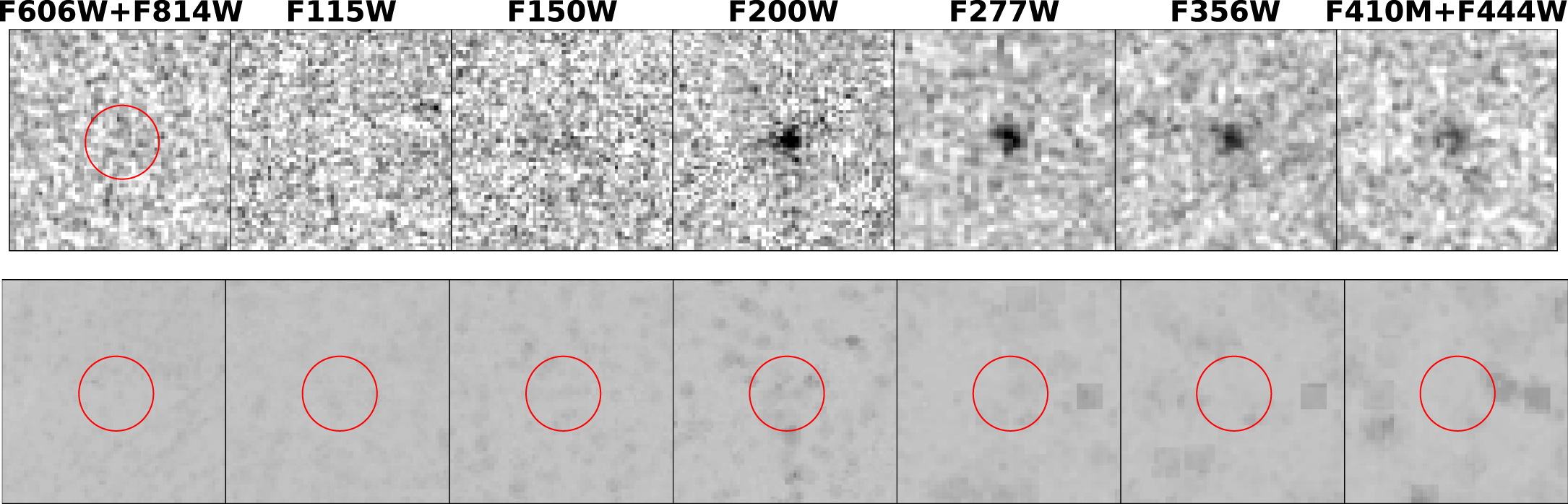
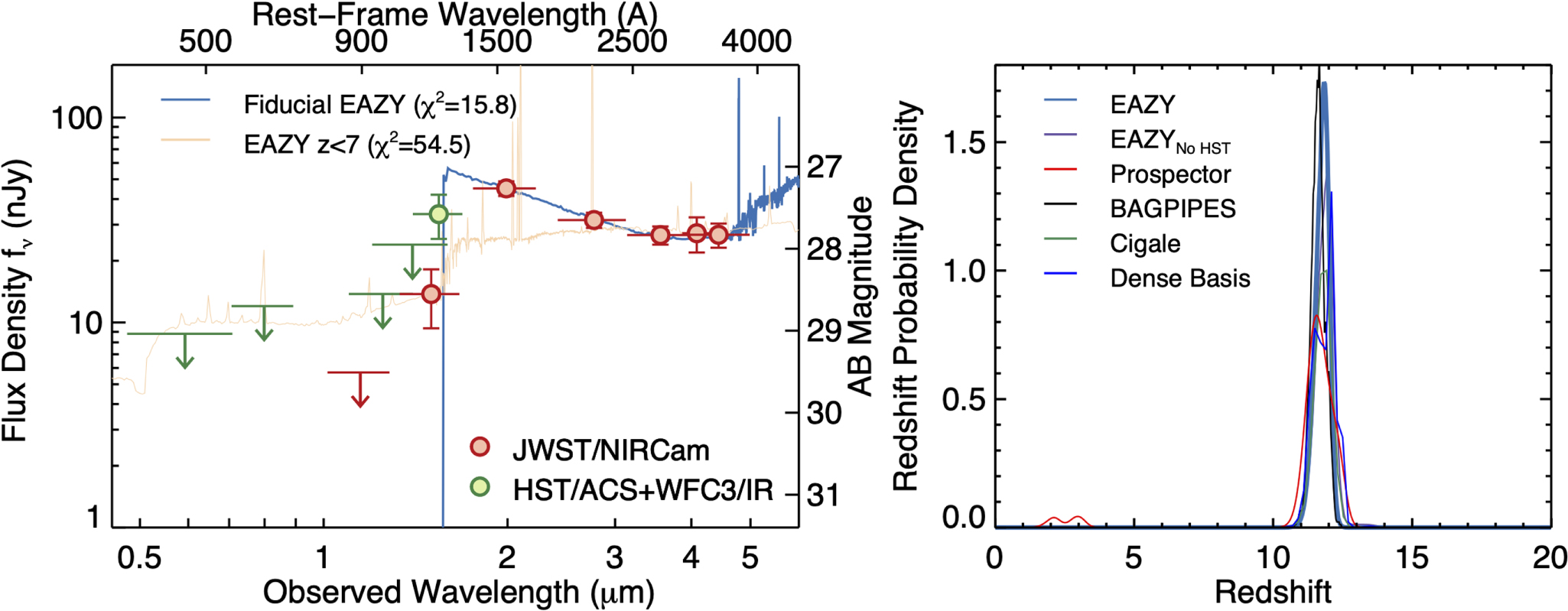
Later spectroscopically confirmed: \(z_\mathrm{spec} = 11.416\) (Arrabal Haro et al. 2023, Nature 622, 711).
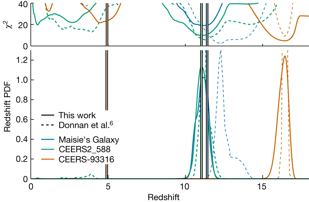
Figure 3: p(z) distribution for sources spectroscopically targeted by Arrabal Haro et al.
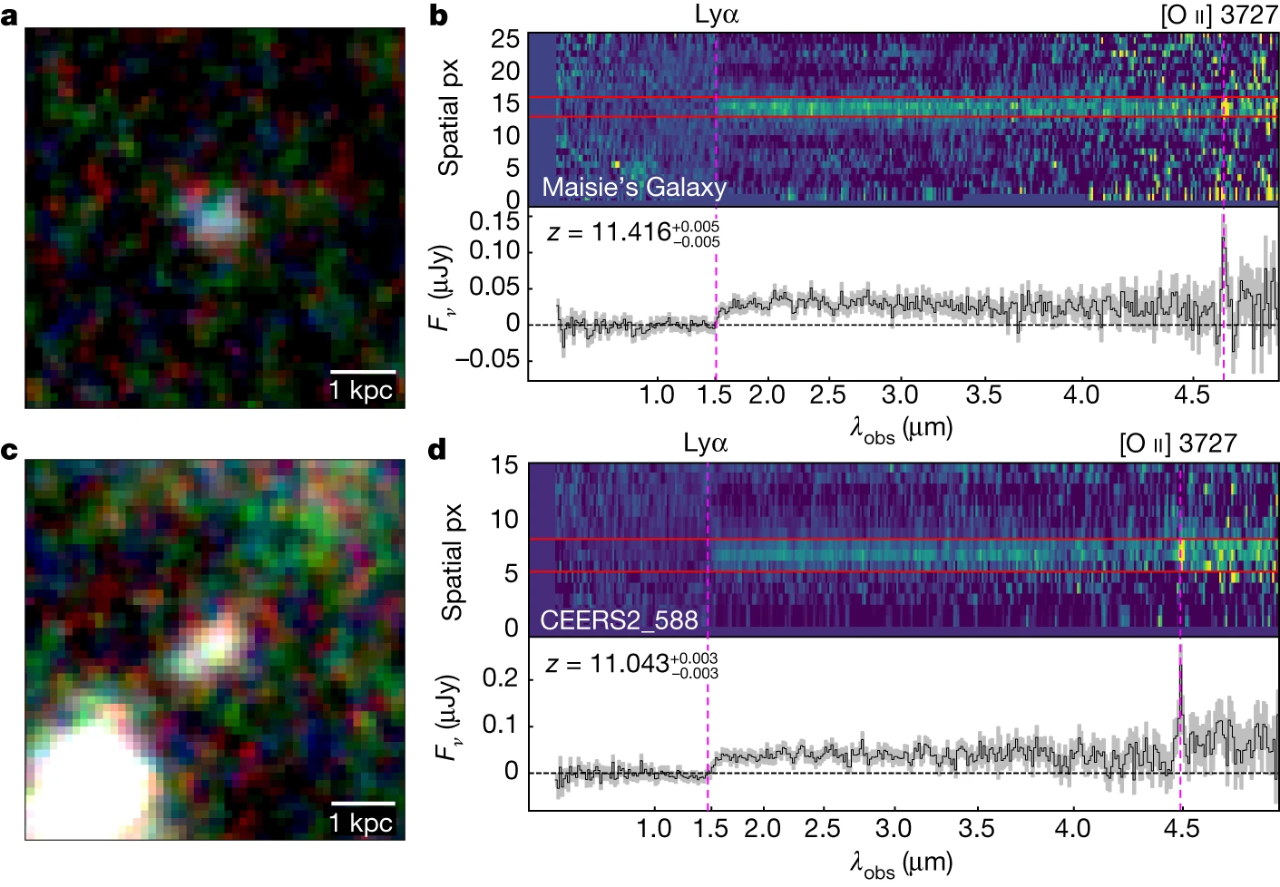
Figure 4: Spectra for z>10 galaxies from Arrabal Haro et al.
3. Spectroscopic Redshifts - Primer
3.1. Astrophysical Emission Lines
HII regions (e.g., Orion). Massive stars ionize surroundings. Recombination and collisions with free electrons produce line spectrum.
Fundamental textbooks describing the basic astrophysics:
- Osterbrock & Ferland (2006): Astrophysics of Gaseous Nebula.
- Aller (1984): Physics of Thermal Gaseous Nebulae.
- …
3.1.1. Principal Lines - optical
| Line | Eᵢₒₙ [eV] | Mechanism | λₐᵢᵣ [Å] |
|---|---|---|---|
| [O II] λ3726 | 13.62 | col | 3726.032 |
| [O II] λ3729 | 13.62 | col | 3728.815 |
| Hδ λ4102 | 13.6 | rec | 4101.735 |
| Hγ λ4341 | 13.6 | rec | 4340.463 |
| Hβ λ4861 | 13.6 | rec | 4861.325 |
| [O III] λ4959 | 35.12 | col | 4958.911 |
| [O III] λ5007 | 35.12 | col | 5006.843 |
| [N II] λ6548 | 14.54 | col | 6548.040 |
| Hα λ6563 | 13.6 | rec | 6562.800 |
| [N II] λ6583 | 14.54 | col | 6583.460 |
| [S II] λ6716 | 10.36 | col | 6716.440 |
| [S II] λ6731 | 10.36 | col | 6730.820 |
- Line: Designation of the line.
- Eᵢₒₙ [eV]; depending on the "Mechanism":
- For collisionally excited lines (col): ionisation potential to create species.
- For recombination lines (rec): ionisation potential to ionise species.
- Wavelengths from https://www.pa.uky.edu/~peter/newpage/ (Van Hoof, P.A.M, Galaxies 2018, 6, 63).
3.1.2. UV Spectral lines (especially Lya).
| Line | Eᵢₒₙ [eV] | Mechanism | λ_vac [Å] |
|---|---|---|---|
| Lyα | 13.62 | rec | 1215.67 |
| HeII | 54.4 | rec | 1640.42 |
| … | … | … | … |
- Lyα is resonant transition. Complex radiative transfer in interstellar- and circum-galactic environments alters not only spatial and spectral morphology of a galaxy's Lyα signal, but also only a fraction of intrinsically (i.e., via recombination) produced Lyα radiation is emitted towards the observer (escape fraction). For more information see book "Lyman-alpha as an Astrophysical and Cosmological Tool".
3.2. Emission Lines from galaxies.
3.2.1. Example: Integrated Spectrum of NGC 7714
From "A Spectrophotometric Atlas of Galaxies" (Kennicut Jr. 1992).
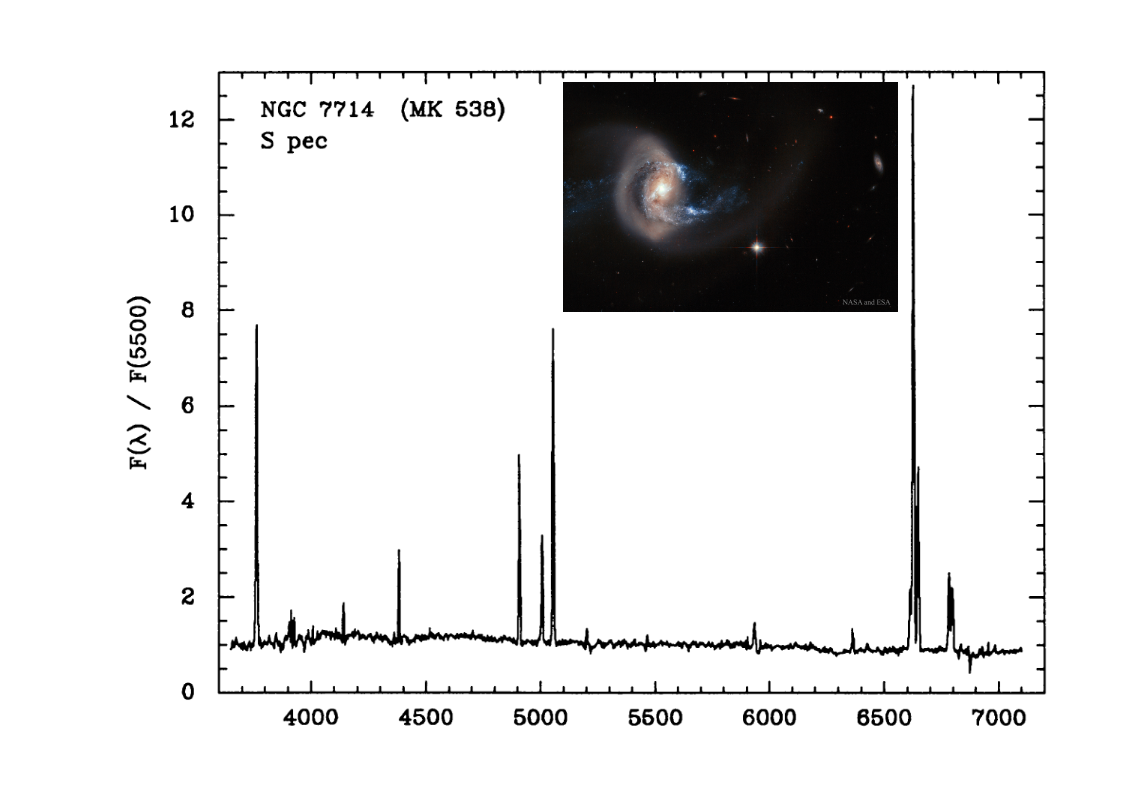
3.2.2. Exercise: Identification of principal lines in the optical in NGC 7714
- Identify the lines from above table in the galaxy spectrum.
- What is the highest redshift that can be measured with an optical spectrograph and the sets of lines in above table?
- Discuss physical processes that create these lines.
- (Discuss physical inferences that are possible from those lines.)
3.2.3. Example: Integrated Spectrum of NGC 1832
- From "A Spectrophotometric Atlas of Galaxies" (Kennicut Jr. 1992).
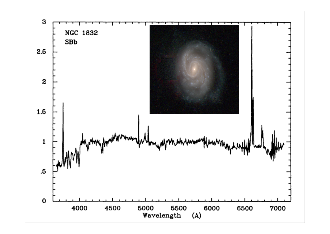 Notice the different line ratios compared to NGC 7714.
(Inset image from Carnegie-Irvine Galaxy Survey.)
3.3. Obtaining Redshifts from Emission Lines
3.3.1. Spectroscopy
Spectrum is 2D. Extraction algorithms needed to produce 1D spectrum.
3.3.2. 1D Spectrum = Input for Redshift Determination
- Numerically: Spectrum = list (1D array) of N flux-density values, sorted by λ, and prescription to convert list (array) index into λ.
- Variance and/or co-variance information are optional.
- Most common data format are FITS files (endorsed by NASA & IAU):
- Container for header-data units.
- Simplest 1D spectrum case: One header-data unit, header contains observational metadata + unit information + prescription to convert array index into λ.
- python support
- via astropy.io.fits module (WCS functionality also accesible via astropy.wcs module).
- astropy affiliated package specutils.
- for modelling spectral features, especially emission lines:
- astropy.modelling (low-level; The Astropy Collaboration et al. 2018)
- LiME (high-level; Fernández et al. 2024)
- astropy.modelling (low-level; The Astropy Collaboration et al. 2018)
3.3.3. Example / Exercise: Extreme Emission Line Galaxies
Inspect the spectra of two extreme emission line galaxies under the following link. By clicking on them an interactive viewer will load. Investigate the difference of plotting the flux on a linear and logartihmic scale. Which spectral features do you recognize?
https://cdsarc.cds.unistra.fr/viz-bin/cat/J/ApJ/938/16 (from Oliver et al. 2022).
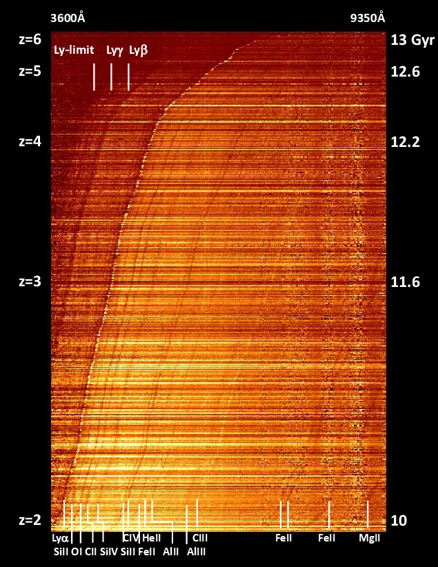
3.3.4. Example: Stack of VUDS 1D spectra sorted by redshift
VUDS = Vimos Ultra Deep Survey
3.3.5. Example: Public Archive of JWST Spectra (DJA)
3.3.6. Readymade solutions
Software solutions exist especially for projects that measure redshifts on industrial scale.
- pyplatefit — https://pyplatefit.readthedocs.io/
- developed as part of MUSE Deep Surveys (Bacon et al. 2023)
- emission and absorption
- requires relatively precise input redshifts
- MarZ (Hinton et al. 2016; contains also an overview of the redshift estimation
software landscape) — "Manual and Automatic Redshifting Software"
- Web application (runs in browser).
- Can be hacked / extended (e.g., special collaboration version used in Bacon et al. 2023)
3.3.7. Underlying principle: Minimization
- Typical solved with non-linear least squares methods.
- Exercise: Fit of a 1D Gaussian(s) to fix redshift of a galaxy.
3.3.7.1. Exercise: Determine Redshift of Source from Spectrum
- Example object from MUSE-Wide Survey (Herenz et al. 2016; Urrutia et al. 2018).
- Object 113004019: https://doi.org/10.17876/musewide/dr.1/113004019
- Local copy of the FITS spectrum from that page: org_attach/e5/13f009-a383-4e6d-b50e-1154b149ad2a/emission_spectrum_candels-cdfs-13_113004019.fits
Use one (ore more) emission lines from the observed spectrum in the FITS file to measure a redshift of this source!
In [3]: hdu.info()
Filename: emission_spectrum_candels-cdfs-13_113004019.fits
No.    Name      Ver    Type      Cards   Dimensions   Format
  0  PRIMARY       1 PrimaryHDU       7   ()
  1                1 BinTableHDU     20   3680R x 4C   [D, D, D, D]
- Solution hint with astropy.modelling
from astropy.io import fits
hdu = fits.open("emission_spectrum_candels-cdfs-13_113004019.fits")
hdu.info()
from astropy.table import Table
t = Table.read("emission_spectrum_candels-cdfs-13_113004019.fits")
t.colnames
wave, flux = t["WAVE_AIR"], t["FLUX"]
from matplotlib import pyplot as plt
plt.plot(wave, flux)
plt.show()
# OIII line is around 6700Å
sel = (wave > 6650.) & (wave < 6750.)
plt.plot(wave[sel], flux[sel])
plt.show()
from astropy.modeling import models

# we use models.Gaussian1D & models.Const1D
cont_model = models.Const1D(amplitude=650)
oiii_model = models.Gaussian1D(
    amplitude=amp_guess - cont_model.amplitude, mean=mean_guess, stddev=stdev_guess
)
# combined model
oiii_cont_model = oiii_model + cont_model

# try making a plot
plt.ion()
plt.plot(wave[sel], flux[sel])
plt.plot(wave[sel], oiii_cont_model(wave[sel]))
Now fit the model!